Nicheverse on Vizgen MERFISH#
Platform. Vizgen MERSCOPE / MERFISH (imaging based, targeted gene panel).
Dataset (real). Mouse retina MERFISH (Vizgen 2023 release), bundled with the package at
examples/data/merfish_retina.h5ad: 113,385 cells x 368 genes, 4 samples. Raw integer counts are in .X, micron
centroids in obsm['spatial'], and obs['sample_id'] holds the four MERFISH runs.
Units. obsm['spatial'] is in microns (the MERFISH global_x / global_y stage
coordinates).
The bundled AnnData ships segmented counts only (no per-molecule table), so this notebook
trains on segmented expression. If you have the Vizgen detected_transcripts.csv
(columns global_x, global_y, gene), you can add a transcript-context input exactly as
in the Xenium notebook by passing platform="merfish". Real runs use about 300 epochs.
import anndata as ad, numpy as np
PLATFORM = "MERFISH (mouse retina)"
adata = ad.read_h5ad("../../examples/data/merfish_retina.h5ad")
assert "spatial" in adata.obsm and "sample_id" in adata.obs
print(adata)
print("samples:", list(adata.obs["sample_id"].unique()),
      "| n_genes:", adata.n_vars,
      "| spatial units ~microns:", adata.obsm["spatial"].max(0).round(0))
AnnData object with n_obs × n_vars = 113385 × 368
    obs: 'sample_id'
    obsm: 'spatial'
samples: ['VZG105a_WT1', 'VZG105a_WT2', 'VZG105a_WT3', 'VZG105a_WT4'] | n_genes: 368 | spatial units ~microns: [8611. 7697.]
Configure and train#
We build a ModelConfig (the architecture) and a TrainConfig (the optimization / spatial graph), then call train_model. The current library default encoder is mlp_deep (a SwiGLU pre-norm residual MLP) with the vq quantizer, and the neighborhood graph is knn_radius (radius 50 um, k = 20). We keep batch_size=2048 rather than 'auto', because an over-large auto batch shrinks the number of optimizer steps per epoch and starves the codebook-diversity term. We run only a handful of demo epochs here so the notebook finishes in minutes; a production run uses about 300 epochs.
import os
from nicheverse.models import ModelConfig, HierarchicalVQVAE
from nicheverse.training import train_model, TrainConfig

ckpt = "runs/nb_merfish_demo"
os.makedirs(ckpt, exist_ok=True)

mc = ModelConfig(
    input_dim=int(adata.n_vars),
    cell_embedding_dim=64, cell_num_embeddings=256,
    neighborhood_embedding_dim=256, neighborhood_num_embeddings=32,
    use_cross_attention=True,
    gene_names=tuple(adata.var_names.astype(str)),
    encoder_type="mlp_plr", quantizer_type="vq",   # strong on a diverse cohort (library default is mlp_deep)
)
tc = TrainConfig(
    num_epochs=30,             # demo; production ~300 (30 epochs already fills ~197/256 codes here)
    batch_size=2048,
    learning_rate=3e-4,
    spatial_graph="knn_radius", radius=50.0, k_neighbors=20,
    normalize=True, log1p=True, seed=9,   # default seed
)
model, adata = train_model(adata, ckpt, model_config=mc, train_config=tc, sample_col="sample_id")
print("done ->", ckpt)
[nicheverse] epoch 1/30 | total=4.4437 cell=1.0278 neigh=3.4159 | perp c/n=6.6/2.1 | active c/n=256/32 | gini c/n=0.96/0.84 | lr=3.00e-04 gnorm=748.27 | 2.3s 49736 cells/s
[nicheverse] epoch 2/30 | total=3.1537 cell=0.3834 neigh=2.7704 | perp c/n=2.5/3.0 | active c/n=20/11 | gini c/n=0.98/0.91 | lr=3.00e-04 gnorm=3.17 | 1.7s 65709 cells/s
[nicheverse] epoch 3/30 | total=1.9644 cell=0.3136 neigh=1.6508 | perp c/n=2.6/6.7 | active c/n=25/9 | gini c/n=0.98/0.82 | lr=3.00e-04 gnorm=0.95 | 1.7s 66241 cells/s
[nicheverse] epoch 4/30 | total=1.8561 cell=0.2912 neigh=1.5649 | perp c/n=2.9/8.1 | active c/n=11/9 | gini c/n=0.98/0.78 | lr=3.00e-04 gnorm=0.50 | 1.7s 66404 cells/s
[nicheverse] epoch 5/30 | total=1.8418 cell=0.2811 neigh=1.5606 | perp c/n=4.7/8.4 | active c/n=8/9 | gini c/n=0.98/0.77 | lr=3.00e-04 gnorm=0.34 | 1.7s 66248 cells/s
[nicheverse] epoch 6/30 | total=1.8322 cell=0.2760 neigh=1.5562 | perp c/n=5.0/8.4 | active c/n=9/9 | gini c/n=0.98/0.77 | lr=3.00e-04 gnorm=0.38 | 1.7s 65405 cells/s
[nicheverse] epoch 7/30 | total=1.7540 cell=0.2723 neigh=1.4817 | perp c/n=2.7/8.9 | active c/n=7/11 | gini c/n=0.99/0.76 | lr=3.00e-04 gnorm=0.41 | 1.7s 66392 cells/s
[nicheverse] epoch 8/30 | total=1.5849 cell=0.2704 neigh=1.3145 | perp c/n=5.4/9.1 | active c/n=9/17 | gini c/n=0.98/0.71 | lr=3.00e-04 gnorm=1.51 | 1.7s 66278 cells/s
[nicheverse] epoch 9/30 | total=1.2170 cell=0.2691 neigh=0.9479 | perp c/n=5.9/11.6 | active c/n=13/25 | gini c/n=0.98/0.63 | lr=3.00e-04 gnorm=2.06 | 1.7s 66256 cells/s
[nicheverse] epoch 10/30 | total=0.9864 cell=0.2673 neigh=0.7191 | perp c/n=22.2/17.1 | active c/n=206/29 | gini c/n=0.92/0.54 | lr=3.00e-04 gnorm=2.07 | 1.7s 66035 cells/s
[nicheverse] epoch 11/30 | total=0.7799 cell=0.2626 neigh=0.5173 | perp c/n=55.1/21.9 | active c/n=175/30 | gini c/n=0.78/0.43 | lr=3.00e-04 gnorm=1.28 | 1.7s 66152 cells/s
[nicheverse] epoch 12/30 | total=0.6688 cell=0.2536 neigh=0.4152 | perp c/n=62.1/24.5 | active c/n=170/32 | gini c/n=0.79/0.34 | lr=3.00e-04 gnorm=1.00 | 1.7s 65825 cells/s
[nicheverse] epoch 13/30 | total=0.5736 cell=0.2495 neigh=0.3241 | perp c/n=83.7/27.5 | active c/n=179/32 | gini c/n=0.73/0.27 | lr=3.00e-04 gnorm=0.99 | 1.7s 66187 cells/s
[nicheverse] epoch 14/30 | total=0.5473 cell=0.2450 neigh=0.3023 | perp c/n=85.6/29.1 | active c/n=170/32 | gini c/n=0.72/0.21 | lr=3.00e-04 gnorm=1.05 | 1.7s 66397 cells/s
[nicheverse] epoch 15/30 | total=0.5335 cell=0.2415 neigh=0.2920 | perp c/n=80.2/29.6 | active c/n=189/32 | gini c/n=0.71/0.18 | lr=3.00e-04 gnorm=0.81 | 1.7s 65933 cells/s
[nicheverse] epoch 16/30 | total=0.5260 cell=0.2392 neigh=0.2868 | perp c/n=83.7/30.1 | active c/n=194/32 | gini c/n=0.73/0.16 | lr=3.00e-04 gnorm=0.72 | 1.7s 66304 cells/s
[nicheverse] epoch 17/30 | total=0.5202 cell=0.2381 neigh=0.2821 | perp c/n=96.4/30.8 | active c/n=199/32 | gini c/n=0.69/0.13 | lr=3.00e-04 gnorm=0.88 | 1.7s 65989 cells/s
[nicheverse] epoch 18/30 | total=0.5155 cell=0.2361 neigh=0.2794 | perp c/n=105.5/31.0 | active c/n=218/32 | gini c/n=0.64/0.12 | lr=3.00e-04 gnorm=0.89 | 1.7s 65857 cells/s
[nicheverse] epoch 19/30 | total=0.5134 cell=0.2366 neigh=0.2768 | perp c/n=103.2/31.1 | active c/n=231/32 | gini c/n=0.64/0.11 | lr=3.00e-04 gnorm=0.73 | 1.7s 66217 cells/s
[nicheverse] epoch 20/30 | total=0.5131 cell=0.2378 neigh=0.2753 | perp c/n=117.1/31.3 | active c/n=214/32 | gini c/n=0.61/0.09 | lr=3.00e-04 gnorm=0.91 | 1.7s 66299 cells/s
[nicheverse] epoch 21/30 | total=0.5112 cell=0.2372 neigh=0.2740 | perp c/n=126.2/31.4 | active c/n=226/32 | gini c/n=0.58/0.08 | lr=3.00e-04 gnorm=1.01 | 1.7s 66634 cells/s
[nicheverse] epoch 22/30 | total=0.5099 cell=0.2369 neigh=0.2729 | perp c/n=132.5/31.4 | active c/n=229/32 | gini c/n=0.56/0.08 | lr=3.00e-04 gnorm=0.99 | 1.7s 66084 cells/s
[nicheverse] epoch 23/30 | total=0.5094 cell=0.2372 neigh=0.2721 | perp c/n=136.3/31.5 | active c/n=231/32 | gini c/n=0.55/0.07 | lr=3.00e-04 gnorm=0.97 | 1.7s 66426 cells/s
[nicheverse] epoch 24/30 | total=0.5104 cell=0.2377 neigh=0.2727 | perp c/n=148.3/31.4 | active c/n=233/32 | gini c/n=0.50/0.08 | lr=3.00e-04 gnorm=1.22 | 1.7s 66331 cells/s
[nicheverse] epoch 25/30 | total=0.5122 cell=0.2390 neigh=0.2732 | perp c/n=158.9/31.3 | active c/n=238/32 | gini c/n=0.47/0.08 | lr=3.00e-04 gnorm=1.23 | 1.7s 66532 cells/s
[nicheverse] epoch 26/30 | total=0.5142 cell=0.2397 neigh=0.2745 | perp c/n=167.4/31.2 | active c/n=248/32 | gini c/n=0.43/0.09 | lr=3.00e-04 gnorm=1.41 | 1.7s 66490 cells/s
[nicheverse] epoch 27/30 | total=0.5141 cell=0.2397 neigh=0.2744 | perp c/n=179.8/31.2 | active c/n=249/32 | gini c/n=0.40/0.09 | lr=3.00e-04 gnorm=1.22 | 1.7s 65932 cells/s
[nicheverse] epoch 28/30 | total=0.5167 cell=0.2406 neigh=0.2761 | perp c/n=188.4/31.2 | active c/n=250/32 | gini c/n=0.36/0.09 | lr=3.00e-04 gnorm=1.27 | 1.7s 65134 cells/s
[nicheverse] epoch 29/30 | total=0.5189 cell=0.2422 neigh=0.2767 | perp c/n=193.1/31.3 | active c/n=253/32 | gini c/n=0.33/0.08 | lr=3.00e-04 gnorm=1.19 | 1.7s 65672 cells/s
[nicheverse] epoch 30/30 | total=0.5184 cell=0.2427 neigh=0.2757 | perp c/n=198.4/31.4 | active c/n=252/32 | gini c/n=0.31/0.08 | lr=1.50e-04 gnorm=1.00 | 1.7s 65831 cells/s
done -> runs/nb_merfish_demo
Inspect the learned codebook#
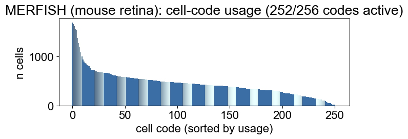
train_model writes the per-cell code assignment to hierarchical_cell_indices.npz (key indices). A well-utilized codebook spreads cells across many codes; a collapsed run concentrates almost all cells in a few codes.
# --- Load the codes the model just assigned to every cell ---
import numpy as np, json, os
idx = np.load(os.path.join(ckpt, "hierarchical_cell_indices.npz"))["indices"].ravel()
n_codes = int(model.config.cell_num_embeddings)
u, counts = np.unique(idx, return_counts=True)
print(f"{PLATFORM}: {len(idx)} cells assigned to {len(u)}/{n_codes} cell codes "
      f"(codebook usage {100*len(u)/n_codes:.0f}%)")
MERFISH (mouse retina): 113385 cells assigned to 252/256 cell codes (codebook usage 98%)
# --- Code-usage bar chart (how many cells fall in each active code) ---
%matplotlib inline
import matplotlib.pyplot as plt
order = np.argsort(counts)[::-1]
fig, ax = plt.subplots(figsize=(7, 3))
ax.bar(range(len(u)), counts[order], color="#3b6ea5")
ax.set_xlabel("cell code (sorted by usage)")
ax.set_ylabel("n cells")
ax.set_title(f"{PLATFORM}: cell-code usage ({len(u)}/{n_codes} codes active)")
plt.tight_layout()
plt.show()
Top markers per code#
For each used code we z-score its mean expression across codes and list the most enriched panel genes. This is a quick biological sanity check that codes track distinct cell states.
# --- Per-code top-marker table: mean log1p expression per code, z-scored across codes ---
import pandas as pd, scanpy as sc
work = adata.copy()
sc.pp.normalize_total(work); sc.pp.log1p(work)
X = work.X.toarray() if hasattr(work.X, "toarray") else np.asarray(work.X)
genes = np.asarray(work.var_names)
rows = []
for c in u:                                   # only codes that are actually used
    m = X[idx == c].mean(0)
    rows.append(m)
M = np.vstack(rows)                            # (n_used_codes, n_genes)
Z = (M - M.mean(0)) / (M.std(0) + 1e-8)        # z across codes, per gene
topk = 6
recs = []
for r, c in enumerate(u):
    top = genes[np.argsort(Z[r])[::-1][:topk]]
    recs.append({"cell_code": int(c), "n_cells": int((idx == c).sum()),
                 "top_markers": ", ".join(top)})
marker_tbl = pd.DataFrame(recs).sort_values("n_cells", ascending=False).reset_index(drop=True)
print(f"Top {topk} enriched genes per used cell code (first 15 codes shown):")
marker_tbl.head(15)
WARNING: adata.X seems to be already log-transformed.
Top 6 enriched genes per used cell code (first 15 codes shown):
| cell_code | n_cells | top_markers | |
|---|---|---|---|
| 0 | 8 | 1682 | Ptk2b, Neurod1, Nr2e3, Prokr1, Tulp1, Reep6 |
| 1 | 44 | 1654 | Tax1bp1, Dmrtb1, Prom1, S100b, Prokr1, Ptk2b |
| 2 | 244 | 1618 | Prom1, Reep6, Neurod1, Nr2e3, Crx, Tulp1 |
| 3 | 232 | 1550 | Prom1, Neurod1, Crx, Reep6, Tulp1, Nr2e3 |
| 4 | 161 | 1539 | Nrl, Dmrtb1, Mfap5, Lmo3, Inadl, Prokr1 |
| 5 | 219 | 1375 | Pde6a, Mafb, Crx, Inadl, Nr2e3, Reep6 |
| 6 | 157 | 1267 | Slc17a7, Reep6, Cngb1, Crx, Neurod1, Prokr1 |
| 7 | 165 | 1201 | Tax1bp1, Dmrtb1, Lima1, 4833423E24Rik, Inadl, ... |
| 8 | 217 | 1076 | Nrl, Pde6a, Tmem114, 4833423E24Rik, Rax, Cxcl13 |
| 9 | 233 | 994 | Tax1bp1, Nrl, Gpr83, Postn, Dmrtb1, Tmem114 |
| 10 | 199 | 933 | Nrl, Prom1, Sfrp2, Ramp3, Mfap5, Neurod1 |
| 11 | 26 | 893 | pla2g7, Ramp3, Hapln1, Prom1, Lyar, Inadl |
| 12 | 255 | 867 | Nrl, Prom1, Bmp2, C1ql3, Neurod1, Nr2e3 |
| 13 | 178 | 853 | Gas7, Anxa3, Tagln2, Neurod1, Tulp1, Nr2e3 |
| 14 | 222 | 818 | Gas7, Prom1, Neurod1, Reep6, Postn, Crx |
Training runtime#
The trainer records wall-clock time, throughput (cells/sec), and peak GPU memory to training_runtime.json.
# --- Training runtime report the trainer wrote (real timing on this GPU run) ---
rt_path = os.path.join(ckpt, "training_runtime.json")
runtime = json.load(open(rt_path))
print(json.dumps(runtime, indent=2))
{
  "total_seconds": 52.039,
  "total_hms": "0:00:52",
  "n_epochs": 30,
  "mean_epoch_seconds": 1.735,
  "cells_per_second": 65366.02,
  "iters_per_second": 32.284,
  "n_cells": 113385,
  "effective_batch_size": 2048,
  "nominal_learning_rate": 0.0003,
  "effective_learning_rate": 0.0003,
  "lr_scaled_with_batch": false,
  "n_batches_per_epoch": 56,
  "peak_gpu_gb": 1.709,
  "device": "cuda",
  "encoder_type": "mlp_plr",
  "quantizer_type": "vq",
  "input_dim": 368
}