Nicheverse on 10x Xenium#
Platform. 10x Genomics Xenium in situ (imaging based, targeted gene panel, subcellular transcript coordinates).
Dataset (real). A single Xenium tissue core from our clear cell renal cell carcinoma (RCC)
cohort, bundled with the package at examples/data/xenium_rcc_core.h5ad: 7,824 cells x 366
panel genes, 1 sample. Raw integer counts are in .X, micron centroids in
obsm['spatial'], and the sample label in obs['sample_id']. The matching molecule table
(subcellular transcript coordinates) is bundled as
examples/data/xenium_rcc_core_transcripts.parquet with columns x_location, y_location,
feature_name (the Xenium convention).
Units. obsm['spatial'] and the molecule coordinates are in microns.
This notebook trains on segmented counts and then shows the optional transcript-context input, which concatenates the segmentation-free local molecular field (molecules within a small radius of each nucleus) onto the segmented counts.
A note on the encoder here. The library default and recommended encoder is mlp_deep,
which stays healthy on sparse Xenium counts. This example is a single fairly homogeneous
RCC core, where 256 codes exceed the core’s intrinsic diversity, so we lower the codebook to
64 codes and use the plain mlp encoder to get a healthy, non-collapsed demo. On the full RCC
Xenium cohort (millions of cells, ~300 epochs) the default mlp_deep with 256 codes is the
recommended setting; per-gene numerical embeddings (mlp_plr) over-parameterize and degenerate
on sparse Xenium panels, so they are not recommended here (they help on diverse gene-rich
cohorts such as the MERFISH retina demo).
import anndata as ad, numpy as np
PLATFORM = "Xenium (RCC core)"
adata = ad.read_h5ad("../../examples/data/xenium_rcc_core.h5ad")
assert "spatial" in adata.obsm and "sample_id" in adata.obs
print(adata)
print("raw counts:", bool(np.all(adata.X[:200].toarray() == np.round(adata.X[:200].toarray()))),
      "| samples:", adata.obs["sample_id"].nunique(),
      "| spatial units ~microns:", adata.obsm["spatial"].max(0).round(0))
AnnData object with n_obs × n_vars = 7824 × 366
    obs: 'sample_id'
    uns: 'source'
    obsm: 'spatial'
raw counts: True | samples: 1 | spatial units ~microns: [11410.  7180.]
Configure and train#
We build a ModelConfig (the architecture) and a TrainConfig (the optimization / spatial graph), then call train_model. The current library default encoder is mlp_deep (a SwiGLU pre-norm residual MLP) with the vq quantizer, and the neighborhood graph is knn_radius (radius 50 um, k = 20). We keep batch_size=2048 rather than 'auto', because an over-large auto batch shrinks the number of optimizer steps per epoch and starves the codebook-diversity term. We run only a handful of demo epochs here so the notebook finishes in minutes; a production run uses about 300 epochs.
import os
from nicheverse.models import ModelConfig, HierarchicalVQVAE
from nicheverse.training import train_model, TrainConfig

ckpt = "runs/nb_xenium_demo"
os.makedirs(ckpt, exist_ok=True)

# The library default and recommended encoder is mlp_deep, which stays healthy on sparse
# Xenium counts. This example is a SINGLE fairly homogeneous RCC core (7,824 cells, 366 genes),
# where 256 codes is far more than one core's intrinsic diversity. So for this small single-core
# demo we lower the codebook to 64 codes and use the plain mlp encoder (verified 64/64 codes
# active). On the full RCC Xenium cohort (millions of cells, ~300 epochs) the default mlp_deep
# with 256 codes is the recommended setting; mlp_plr (per-gene numerical embeddings) degenerates
# on sparse Xenium panels and is not recommended here.
mc = ModelConfig(
    input_dim=int(adata.n_vars),
    cell_embedding_dim=64, cell_num_embeddings=64,   # 64 codes for one small core
    neighborhood_embedding_dim=256, neighborhood_num_embeddings=16,
    use_cross_attention=True,
    gene_names=tuple(adata.var_names.astype(str)),
    encoder_type="mlp",         # collapse-resistant on a single small core
    quantizer_type="vq",        # library default
)
tc = TrainConfig(
    num_epochs=40,              # demo; production ~300
    batch_size=2048,            # NOT 'auto' (protects codebook diversity)
    learning_rate=3e-4,
    spatial_graph="knn_radius", radius=50.0, k_neighbors=20,  # library defaults
    normalize=True, log1p=True, seed=9,
)
model, adata = train_model(adata, ckpt, model_config=mc, train_config=tc, sample_col="sample_id")
print("done ->", ckpt)
[nicheverse] epoch 1/40 | total=4.1464 cell=2.1323 neigh=2.0141 | perp c/n=18.6/6.4 | active c/n=64/16 | gini c/n=0.76/0.69 | lr=3.00e-04 gnorm=3.51 | 0.4s 19244 cells/s
[nicheverse] epoch 2/40 | total=3.5453 cell=1.8397 neigh=1.7055 | perp c/n=26.7/7.9 | active c/n=58/13 | gini c/n=0.68/0.57 | lr=3.00e-04 gnorm=2.06 | 0.1s 103053 cells/s
[nicheverse] epoch 3/40 | total=3.1788 cell=1.6546 neigh=1.5242 | perp c/n=31.3/8.9 | active c/n=57/14 | gini c/n=0.59/0.53 | lr=3.00e-04 gnorm=1.52 | 0.1s 105883 cells/s
[nicheverse] epoch 4/40 | total=2.9440 cell=1.5549 neigh=1.3890 | perp c/n=33.1/9.8 | active c/n=55/14 | gini c/n=0.57/0.46 | lr=3.00e-04 gnorm=1.35 | 0.1s 108038 cells/s
[nicheverse] epoch 5/40 | total=2.7844 cell=1.4640 neigh=1.3203 | perp c/n=34.6/10.2 | active c/n=57/15 | gini c/n=0.55/0.43 | lr=3.00e-04 gnorm=1.28 | 0.1s 107986 cells/s
[nicheverse] epoch 6/40 | total=2.6242 cell=1.3791 neigh=1.2451 | perp c/n=36.4/10.7 | active c/n=56/14 | gini c/n=0.53/0.39 | lr=3.00e-04 gnorm=1.26 | 0.1s 109630 cells/s
[nicheverse] epoch 7/40 | total=2.4808 cell=1.2731 neigh=1.2078 | perp c/n=40.1/10.9 | active c/n=58/15 | gini c/n=0.49/0.37 | lr=3.00e-04 gnorm=1.06 | 0.1s 108900 cells/s
[nicheverse] epoch 8/40 | total=2.3776 cell=1.1946 neigh=1.1830 | perp c/n=42.7/11.0 | active c/n=58/15 | gini c/n=0.43/0.36 | lr=3.00e-04 gnorm=1.06 | 0.1s 102390 cells/s
[nicheverse] epoch 9/40 | total=2.2898 cell=1.1339 neigh=1.1559 | perp c/n=44.7/11.1 | active c/n=62/15 | gini c/n=0.40/0.35 | lr=3.00e-04 gnorm=0.97 | 0.1s 108595 cells/s
[nicheverse] epoch 10/40 | total=2.2002 cell=1.0743 neigh=1.1260 | perp c/n=46.8/11.3 | active c/n=60/15 | gini c/n=0.37/0.35 | lr=3.00e-04 gnorm=1.13 | 0.1s 107847 cells/s
[nicheverse] epoch 11/40 | total=2.0955 cell=1.0245 neigh=1.0710 | perp c/n=48.3/11.8 | active c/n=58/15 | gini c/n=0.33/0.33 | lr=3.00e-04 gnorm=1.05 | 0.1s 108472 cells/s
[nicheverse] epoch 12/40 | total=1.9963 cell=0.9883 neigh=1.0080 | perp c/n=49.4/12.6 | active c/n=60/16 | gini c/n=0.31/0.28 | lr=3.00e-04 gnorm=1.10 | 0.1s 108416 cells/s
[nicheverse] epoch 13/40 | total=1.9089 cell=0.9435 neigh=0.9654 | perp c/n=50.6/13.0 | active c/n=63/16 | gini c/n=0.29/0.24 | lr=3.00e-04 gnorm=0.93 | 0.2s 50413 cells/s
[nicheverse] epoch 14/40 | total=1.8417 cell=0.8998 neigh=0.9419 | perp c/n=52.3/13.2 | active c/n=64/16 | gini c/n=0.28/0.23 | lr=3.00e-04 gnorm=1.05 | 0.1s 103661 cells/s
[nicheverse] epoch 15/40 | total=1.7614 cell=0.8697 neigh=0.8917 | perp c/n=52.9/13.9 | active c/n=64/16 | gini c/n=0.28/0.21 | lr=3.00e-04 gnorm=1.32 | 0.1s 104973 cells/s
[nicheverse] epoch 16/40 | total=1.6425 cell=0.8131 neigh=0.8294 | perp c/n=55.2/14.7 | active c/n=64/16 | gini c/n=0.25/0.15 | lr=3.00e-04 gnorm=0.92 | 0.1s 100497 cells/s
[nicheverse] epoch 17/40 | total=1.6018 cell=0.7735 neigh=0.8283 | perp c/n=57.4/14.6 | active c/n=63/16 | gini c/n=0.20/0.18 | lr=3.00e-04 gnorm=0.79 | 0.1s 100273 cells/s
[nicheverse] epoch 18/40 | total=1.5649 cell=0.7471 neigh=0.8178 | perp c/n=59.1/14.7 | active c/n=64/16 | gini c/n=0.17/0.17 | lr=3.00e-04 gnorm=0.74 | 0.1s 104068 cells/s
[nicheverse] epoch 19/40 | total=1.5258 cell=0.7254 neigh=0.8004 | perp c/n=59.9/14.9 | active c/n=64/16 | gini c/n=0.17/0.12 | lr=3.00e-04 gnorm=0.56 | 0.1s 100792 cells/s
[nicheverse] epoch 20/40 | total=1.5091 cell=0.7107 neigh=0.7984 | perp c/n=60.3/14.9 | active c/n=64/15 | gini c/n=0.14/0.12 | lr=3.00e-04 gnorm=0.56 | 0.1s 100820 cells/s
[nicheverse] epoch 21/40 | total=1.4890 cell=0.6969 neigh=0.7922 | perp c/n=61.1/14.9 | active c/n=64/16 | gini c/n=0.12/0.10 | lr=3.00e-04 gnorm=0.45 | 0.1s 107711 cells/s
[nicheverse] epoch 22/40 | total=1.4726 cell=0.6866 neigh=0.7859 | perp c/n=61.2/15.0 | active c/n=64/16 | gini c/n=0.13/0.08 | lr=3.00e-04 gnorm=0.42 | 0.1s 108206 cells/s
[nicheverse] epoch 23/40 | total=1.4609 cell=0.6777 neigh=0.7832 | perp c/n=61.3/15.0 | active c/n=64/16 | gini c/n=0.12/0.09 | lr=3.00e-04 gnorm=0.49 | 0.1s 108413 cells/s
[nicheverse] epoch 24/40 | total=1.4533 cell=0.6716 neigh=0.7817 | perp c/n=61.3/15.0 | active c/n=64/16 | gini c/n=0.12/0.10 | lr=3.00e-04 gnorm=0.39 | 0.1s 105507 cells/s
[nicheverse] epoch 25/40 | total=1.4387 cell=0.6624 neigh=0.7762 | perp c/n=61.8/15.0 | active c/n=64/16 | gini c/n=0.11/0.09 | lr=3.00e-04 gnorm=0.44 | 0.1s 107888 cells/s
[nicheverse] epoch 26/40 | total=1.4256 cell=0.6548 neigh=0.7708 | perp c/n=62.4/15.1 | active c/n=64/16 | gini c/n=0.09/0.09 | lr=3.00e-04 gnorm=0.53 | 0.1s 108737 cells/s
[nicheverse] epoch 27/40 | total=1.4097 cell=0.6493 neigh=0.7604 | perp c/n=62.5/15.2 | active c/n=64/16 | gini c/n=0.08/0.08 | lr=3.00e-04 gnorm=0.45 | 0.1s 107777 cells/s
[nicheverse] epoch 28/40 | total=1.3920 cell=0.6460 neigh=0.7460 | perp c/n=62.5/15.4 | active c/n=64/16 | gini c/n=0.08/0.07 | lr=3.00e-04 gnorm=0.66 | 0.1s 102712 cells/s
[nicheverse] epoch 29/40 | total=1.3630 cell=0.6433 neigh=0.7197 | perp c/n=62.7/15.8 | active c/n=64/16 | gini c/n=0.07/0.05 | lr=3.00e-04 gnorm=0.35 | 0.1s 107337 cells/s
[nicheverse] epoch 30/40 | total=1.3542 cell=0.6417 neigh=0.7125 | perp c/n=62.6/15.9 | active c/n=64/16 | gini c/n=0.07/0.04 | lr=3.00e-04 gnorm=0.30 | 0.1s 108020 cells/s
[nicheverse] epoch 31/40 | total=1.3502 cell=0.6383 neigh=0.7119 | perp c/n=62.6/15.9 | active c/n=64/16 | gini c/n=0.08/0.05 | lr=3.00e-04 gnorm=0.31 | 0.1s 108252 cells/s
[nicheverse] epoch 32/40 | total=1.3460 cell=0.6360 neigh=0.7099 | perp c/n=62.4/15.9 | active c/n=64/16 | gini c/n=0.08/0.05 | lr=3.00e-04 gnorm=0.32 | 0.1s 106812 cells/s
[nicheverse] epoch 33/40 | total=1.3408 cell=0.6337 neigh=0.7071 | perp c/n=62.6/15.9 | active c/n=64/16 | gini c/n=0.08/0.04 | lr=3.00e-04 gnorm=0.29 | 0.1s 104222 cells/s
[nicheverse] epoch 34/40 | total=1.3379 cell=0.6330 neigh=0.7050 | perp c/n=62.6/15.9 | active c/n=64/16 | gini c/n=0.07/0.02 | lr=3.00e-04 gnorm=0.27 | 0.1s 103290 cells/s
[nicheverse] epoch 35/40 | total=1.3342 cell=0.6293 neigh=0.7049 | perp c/n=62.6/15.9 | active c/n=64/16 | gini c/n=0.08/0.02 | lr=3.00e-04 gnorm=0.24 | 0.1s 105464 cells/s
[nicheverse] epoch 36/40 | total=1.3308 cell=0.6279 neigh=0.7029 | perp c/n=62.5/15.9 | active c/n=64/16 | gini c/n=0.07/0.02 | lr=3.00e-04 gnorm=0.26 | 0.1s 104310 cells/s
[nicheverse] epoch 37/40 | total=1.3283 cell=0.6260 neigh=0.7023 | perp c/n=62.6/16.0 | active c/n=64/16 | gini c/n=0.07/0.02 | lr=3.00e-04 gnorm=0.23 | 0.1s 104686 cells/s
[nicheverse] epoch 38/40 | total=1.3245 cell=0.6239 neigh=0.7006 | perp c/n=62.8/16.0 | active c/n=64/16 | gini c/n=0.06/0.02 | lr=3.00e-04 gnorm=0.25 | 0.1s 106644 cells/s
[nicheverse] epoch 39/40 | total=1.3227 cell=0.6235 neigh=0.6992 | perp c/n=62.5/16.0 | active c/n=64/16 | gini c/n=0.06/0.02 | lr=3.00e-04 gnorm=0.25 | 0.1s 107702 cells/s
[nicheverse] epoch 40/40 | total=1.3211 cell=0.6216 neigh=0.6994 | perp c/n=62.6/15.9 | active c/n=64/16 | gini c/n=0.08/0.02 | lr=3.00e-04 gnorm=0.25 | 0.1s 105053 cells/s
done -> runs/nb_xenium_demo
Optional: transcript-context input#
Xenium ships subcellular transcript coordinates, so we can build the segmentation-free molecular field and attach it as an obsm matrix. This is the input used in notebooks/02_transcript_context.ipynb.
# --- Optional: transcript-context input (segmentation-free molecular field) ---
# Xenium is one of the platforms with a real per-cell molecule table bundled, so we can
# demonstrate transcript_context here. It adds an obsm matrix of local molecule counts
# (radius 7 um around each nucleus centroid) that can be concatenated onto segmented counts.
from nicheverse.data.transcript import transcript_context
feats = transcript_context(
    adata,
    transcripts="../../examples/data/xenium_rcc_core_transcripts.parquet",
    radius=7.0, platform="xenium", sample_col="sample_id",
    key_added="transcript_context",
)
print("transcript_context obsm shape:", adata.obsm["transcript_context"].shape,
      "| nonzero cells:", int((adata.obsm["transcript_context"].sum(1) > 0).sum()))
# To train on the joint representation, concatenate counts + field into X and set
# input_dim = 2 * n_genes (see notebooks/02_transcript_context.ipynb for the full recipe).
transcript_context obsm shape: (7824, 366) | nonzero cells: 7824
Inspect the learned codebook#
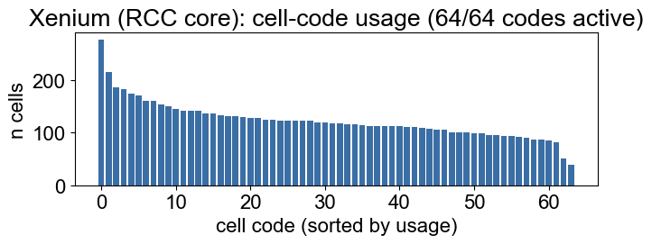
train_model writes the per-cell code assignment to hierarchical_cell_indices.npz (key indices). A well-utilized codebook spreads cells across many codes; a collapsed run concentrates almost all cells in a few codes.
# --- Load the codes the model just assigned to every cell ---
import numpy as np, json, os
idx = np.load(os.path.join(ckpt, "hierarchical_cell_indices.npz"))["indices"].ravel()
n_codes = int(model.config.cell_num_embeddings)
u, counts = np.unique(idx, return_counts=True)
print(f"{PLATFORM}: {len(idx)} cells assigned to {len(u)}/{n_codes} cell codes "
      f"(codebook usage {100*len(u)/n_codes:.0f}%)")
Xenium (RCC core): 7824 cells assigned to 64/64 cell codes (codebook usage 100%)
# --- Code-usage bar chart (how many cells fall in each active code) ---
%matplotlib inline
import matplotlib.pyplot as plt
order = np.argsort(counts)[::-1]
fig, ax = plt.subplots(figsize=(7, 3))
ax.bar(range(len(u)), counts[order], color="#3b6ea5")
ax.set_xlabel("cell code (sorted by usage)")
ax.set_ylabel("n cells")
ax.set_title(f"{PLATFORM}: cell-code usage ({len(u)}/{n_codes} codes active)")
plt.tight_layout()
plt.show()
Top markers per code#
For each used code we z-score its mean expression across codes and list the most enriched panel genes. This is a quick biological sanity check that codes track distinct cell states.
# --- Per-code top-marker table: mean log1p expression per code, z-scored across codes ---
import pandas as pd, scanpy as sc
work = adata.copy()
sc.pp.normalize_total(work); sc.pp.log1p(work)
X = work.X.toarray() if hasattr(work.X, "toarray") else np.asarray(work.X)
genes = np.asarray(work.var_names)
rows = []
for c in u:                                   # only codes that are actually used
    m = X[idx == c].mean(0)
    rows.append(m)
M = np.vstack(rows)                            # (n_used_codes, n_genes)
Z = (M - M.mean(0)) / (M.std(0) + 1e-8)        # z across codes, per gene
topk = 6
recs = []
for r, c in enumerate(u):
    top = genes[np.argsort(Z[r])[::-1][:topk]]
    recs.append({"cell_code": int(c), "n_cells": int((idx == c).sum()),
                 "top_markers": ", ".join(top)})
marker_tbl = pd.DataFrame(recs).sort_values("n_cells", ascending=False).reset_index(drop=True)
print(f"Top {topk} enriched genes per used cell code (first 15 codes shown):")
marker_tbl.head(15)
WARNING: adata.X seems to be already log-transformed.
Top 6 enriched genes per used cell code (first 15 codes shown):
| cell_code | n_cells | top_markers | |
|---|---|---|---|
| 0 | 37 | 276 | PVALB, CDH1, ADAMTS16, KLK6, L1CAM, MYRF |
| 1 | 1 | 215 | SOX9, C1QL3, L1CAM, CDKN1A, NTNG1, MGST1 |
| 2 | 2 | 186 | FGFR3, CAPN3, MYRF, CDH1, SOX4, CA9 |
| 3 | 57 | 182 | LAG3, TNFSF4, NKG7, GZMB, IFNG, CCL4 |
| 4 | 35 | 174 | TREM2, CD14, GPNMB, MAFB, CD163, CD68 |
| 5 | 11 | 170 | TESPA1, CDKN1B, CORO1A, BRINP3, THEMIS, CDH12 |
| 6 | 56 | 161 | KLRD1, KLRC1, MCTP2, GZMB, GNLY, HAVCR2 |
| 7 | 3 | 161 | LHX6, LYVE1, PLVAP, FOLH1, KDR, FLT4 |
| 8 | 58 | 153 | CITED1, OSR1, TTYH1, SORCS1, RORB, OPALIN |
| 9 | 41 | 150 | ADAMTS12, LAMA2, TRIL, TSHZ2, THSD4, UNC5B |
| 10 | 46 | 145 | IL2RA, IKZF2, FOXP3, NR4A2, CTLA4, CD80 |
| 11 | 15 | 142 | IGFBP5, ADAMTS12, THSD4, CLDN11, SPON1, NPFFR2 |
| 12 | 36 | 141 | CD36, ITGAM, TREM2, C1orf162, MAFB, SPI1 |
| 13 | 10 | 141 | CCR7, PSENEN, OLIG1, CD83, FOXP3, CPA3 |
| 14 | 30 | 136 | NPNT, TGFB2, FILIP1, COL12A1, CSPG4, SLIT3 |
Training runtime#
The trainer records wall-clock time, throughput (cells/sec), and peak GPU memory to training_runtime.json.
# --- Training runtime report the trainer wrote (real timing on this GPU run) ---
rt_path = os.path.join(ckpt, "training_runtime.json")
runtime = json.load(open(rt_path))
print(json.dumps(runtime, indent=2))
{
  "total_seconds": 3.397,
  "total_hms": "0:00:03",
  "n_epochs": 40,
  "mean_epoch_seconds": 0.085,
  "cells_per_second": 92129.26,
  "iters_per_second": 47.101,
  "n_cells": 7824,
  "effective_batch_size": 2048,
  "nominal_learning_rate": 0.0003,
  "effective_learning_rate": 0.0003,
  "lr_scaled_with_batch": false,
  "n_batches_per_epoch": 4,
  "peak_gpu_gb": 0.238,
  "device": "cuda",
  "encoder_type": "mlp",
  "quantizer_type": "vq",
  "input_dim": 366
}