06 Downstream analysis: using the codes and embeddings#
Training attaches four things to your AnnData: the discrete cell_codebook_idx and
neighborhood_codebook_idx, and the continuous X_cell_embedding /
X_neighborhood_embedding. This notebook shows the three things you most often do
with them, all with standard scanpy / pandas:
a UMAP of the continuous cell embedding, colored by cell code;
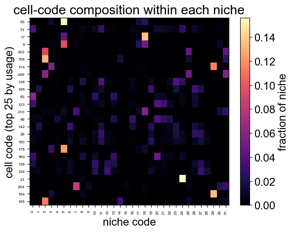
the cell-code x niche composition, which is how the two codebooks connect (which cell states populate which tissue niches);
per-sample code usage.
Everything here is offline and deterministic.
import os
import numpy as np, pandas as pd
import scanpy as sc
import nicheverse as nv
from nicheverse import ModelConfig, TrainConfig
DATA = os.path.join('..', 'examples', 'data')

adata = nv.read_spatial(os.path.join(DATA, 'merfish_retina.h5ad'), sample_col='sample_id')
mc = ModelConfig(input_dim=adata.n_vars, gene_names=tuple(adata.var_names.astype(str)),
                 encoder_type='mlp_deep', cell_num_embeddings=256, neighborhood_num_embeddings=32)
tc = TrainConfig(num_epochs=15, batch_size=2048, spatial_graph='knn_radius', radius=50.0,
                 k_neighbors=20, save_best=False, seed=9)
model, adata = nv.train_model(adata, 'runs/downstream_demo', model_config=mc, train_config=tc,
                              sample_col='sample_id')
print(nv.anndata_keys())
print('embedding:', adata.obsm['X_cell_embedding'].shape)
[nicheverse] epoch 1/15 | total=1.6397 cell=0.9279 neigh=0.7118 | perp c/n=171.5/24.9 | active c/n=256/32 | gini c/n=0.23/0.16 | lr=3.00e-04 gnorm=6.16 | 2.1s 54313 cells/s
[nicheverse] epoch 2/15 | total=0.8889 cell=0.4577 neigh=0.4312 | perp c/n=226.8/29.5 | active c/n=256/31 | gini c/n=0.07/0.08 | lr=3.00e-04 gnorm=2.45 | 1.6s 72145 cells/s
[nicheverse] epoch 3/15 | total=0.7604 cell=0.3649 neigh=0.3954 | perp c/n=233.8/29.5 | active c/n=256/31 | gini c/n=0.04/0.07 | lr=3.00e-04 gnorm=2.41 | 1.6s 71322 cells/s
[nicheverse] epoch 4/15 | total=0.7011 cell=0.3269 neigh=0.3741 | perp c/n=234.7/29.5 | active c/n=256/31 | gini c/n=0.05/0.07 | lr=3.00e-04 gnorm=2.37 | 1.6s 72164 cells/s
[nicheverse] epoch 5/15 | total=0.6394 cell=0.3050 neigh=0.3345 | perp c/n=233.5/30.4 | active c/n=256/31 | gini c/n=0.07/0.04 | lr=3.00e-04 gnorm=2.20 | 1.6s 72095 cells/s
[nicheverse] epoch 6/15 | total=0.6143 cell=0.2869 neigh=0.3275 | perp c/n=232.9/30.4 | active c/n=256/31 | gini c/n=0.08/0.04 | lr=3.00e-04 gnorm=2.17 | 1.6s 71754 cells/s
[nicheverse] epoch 7/15 | total=0.5962 cell=0.2764 neigh=0.3199 | perp c/n=231.2/30.5 | active c/n=256/31 | gini c/n=0.10/0.04 | lr=3.00e-04 gnorm=1.99 | 1.6s 71739 cells/s
[nicheverse] epoch 8/15 | total=0.5888 cell=0.2690 neigh=0.3198 | perp c/n=231.2/30.4 | active c/n=256/31 | gini c/n=0.10/0.04 | lr=3.00e-04 gnorm=2.07 | 1.6s 71654 cells/s
[nicheverse] epoch 9/15 | total=0.5792 cell=0.2633 neigh=0.3159 | perp c/n=231.3/30.5 | active c/n=256/31 | gini c/n=0.11/0.04 | lr=3.00e-04 gnorm=1.84 | 1.6s 71624 cells/s
[nicheverse] epoch 10/15 | total=0.5706 cell=0.2597 neigh=0.3109 | perp c/n=232.2/30.6 | active c/n=256/32 | gini c/n=0.10/0.04 | lr=3.00e-04 gnorm=1.70 | 1.6s 71752 cells/s
[nicheverse] epoch 11/15 | total=0.5429 cell=0.2587 neigh=0.2842 | perp c/n=231.6/31.5 | active c/n=256/32 | gini c/n=0.10/0.01 | lr=3.00e-04 gnorm=1.73 | 1.6s 71380 cells/s
[nicheverse] epoch 12/15 | total=0.5422 cell=0.2565 neigh=0.2857 | perp c/n=232.0/31.4 | active c/n=256/32 | gini c/n=0.10/0.01 | lr=3.00e-04 gnorm=2.00 | 1.6s 71260 cells/s
[nicheverse] epoch 13/15 | total=0.5377 cell=0.2545 neigh=0.2831 | perp c/n=232.8/31.5 | active c/n=256/32 | gini c/n=0.10/0.01 | lr=3.00e-04 gnorm=1.80 | 1.6s 71969 cells/s
[nicheverse] epoch 14/15 | total=0.5349 cell=0.2540 neigh=0.2809 | perp c/n=232.8/31.5 | active c/n=256/32 | gini c/n=0.10/0.01 | lr=3.00e-04 gnorm=1.74 | 1.6s 71436 cells/s
[nicheverse] epoch 15/15 | total=0.5322 cell=0.2519 neigh=0.2804 | perp c/n=233.2/31.5 | active c/n=256/32 | gini c/n=0.09/0.01 | lr=3.00e-04 gnorm=1.60 | 1.6s 71644 cells/s
{'cell_code': 'cell_codebook_idx', 'neighborhood_code': 'neighborhood_codebook_idx', 'sample': 'sample_id', 'cell_embedding': 'X_cell_embedding', 'neighborhood_embedding': 'X_neighborhood_embedding', 'spatial': 'spatial'}
embedding: (113385, 64)
1. A 2D map of the cell embedding#
The continuous embedding is a drop-in use_rep for the standard scanpy neighbors +
UMAP. We try UMAP and fall back to a 2D PCA if umap-learn is unavailable, so the
cell runs in any environment. Coloring by cell_codebook_idx shows that the discrete
codes carve the embedding into coherent regions.
%matplotlib inline
import matplotlib.pyplot as plt   # after importing nicheverse (which selects Agg), re-assert inline
emb = np.asarray(adata.obsm['X_cell_embedding'])
try:
    sc.pp.neighbors(adata, use_rep='X_cell_embedding', n_neighbors=15)
    sc.tl.umap(adata)
    xy = adata.obsm['X_umap']; method = 'UMAP'
except Exception as e:
    from sklearn.decomposition import PCA
    xy = PCA(n_components=2, random_state=0).fit_transform(emb); method = 'PCA'
    print('umap-learn unavailable, using 2D PCA instead:', type(e).__name__)
codes = adata.obs['cell_codebook_idx'].to_numpy()
fig, ax = plt.subplots(figsize=(5.2, 4.4))
ax.scatter(xy[:, 0], xy[:, 1], c=codes, s=2, cmap='tab20', linewidths=0)
ax.set_xlabel(f'{method}1'); ax.set_ylabel(f'{method}2')
ax.set_title(f'cell embedding ({method}), colored by cell code')
ax.set_xticks([]); ax.set_yticks([])
fig.tight_layout(); plt.show()
print('cells:', adata.n_obs, ' distinct cell codes:', len(np.unique(codes)))
---------------------------------------------------------------------------
AttributeError                            Traceback (most recent call last)
AttributeError: _ARRAY_API not found
---------------------------------------------------------------------------
AttributeError                            Traceback (most recent call last)
AttributeError: _ARRAY_API not found
---------------------------------------------------------------------------
ImportError                               Traceback (most recent call last)
ImportError: numpy.core._multiarray_umath failed to import
---------------------------------------------------------------------------
ImportError                               Traceback (most recent call last)
ImportError: numpy.core.umath failed to import
umap-learn unavailable, using 2D PCA instead: TypeError
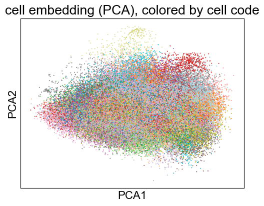
cells: 113385 distinct cell codes: 256
2. Cell-code x niche composition#
This is the join between the two codebooks: for each niche, what mixture of cell codes lives there. A block structure means niches are stereotyped (each recurs with a characteristic cell-code composition), which is what makes the niche codebook a map of tissue organization.
comp = pd.crosstab(adata.obs['cell_codebook_idx'], adata.obs['neighborhood_codebook_idx'])
comp = comp.div(comp.sum(0), axis=1)  # column-normalize: composition within each niche
top_codes = comp.sum(1).sort_values(ascending=False).head(25).index
M = comp.loc[top_codes]
fig, ax = plt.subplots(figsize=(6.2, 5.0))
im = ax.imshow(M.values, aspect='auto', cmap='magma')
ax.set_xlabel('niche code'); ax.set_ylabel('cell code (top 25 by usage)')
ax.set_title('cell-code composition within each niche')
ax.set_xticks(range(M.shape[1])); ax.set_xticklabels(M.columns, fontsize=6, rotation=90)
ax.set_yticks(range(M.shape[0])); ax.set_yticklabels(M.index, fontsize=6)
fig.colorbar(im, ax=ax, fraction=0.046, label='fraction of niche')
fig.tight_layout(); plt.show()
3. Per-sample code usage#
A quick check that the codebook is shared across samples rather than one code per sample. Each row is a sample; each column a cell code; the value is the fraction of that sample’s cells in the code.
usage = pd.crosstab(adata.obs['sample_id'], adata.obs['cell_codebook_idx'], normalize='index')
print('samples:', usage.shape[0], ' codes:', usage.shape[1])
usage.iloc[:, :12].round(3)
samples: 4 codes: 256
| cell_codebook_idx | 0 | 1 | 2 | 3 | 4 | 5 | 6 | 7 | 8 | 9 | 10 | 11 |
|---|---|---|---|---|---|---|---|---|---|---|---|---|
| sample_id | ||||||||||||
| VZG105a_WT1 | 0.008 | 0.002 | 0.002 | 0.002 | 0.002 | 0.005 | 0.003 | 0.007 | 0.004 | 0.002 | 0.006 | 0.001 |
| VZG105a_WT2 | 0.005 | 0.004 | 0.002 | 0.005 | 0.003 | 0.001 | 0.001 | 0.003 | 0.005 | 0.006 | 0.004 | 0.005 |
| VZG105a_WT3 | 0.002 | 0.001 | 0.002 | 0.004 | 0.002 | 0.006 | 0.003 | 0.006 | 0.004 | 0.006 | 0.002 | 0.002 |
| VZG105a_WT4 | 0.004 | 0.002 | 0.003 | 0.005 | 0.002 | 0.003 | 0.003 | 0.002 | 0.004 | 0.005 | 0.004 | 0.008 |
Takeaways#
The continuous embeddings plug straight into the scanpy neighbors / UMAP / clustering stack; the discrete codes are a ready-made categorical for coloring and grouping.
The cell-code x niche crosstab is the bridge between the two codebooks and the starting point for compositional and enrichment analyses (for example, testing whether a cell state is enriched in a particular niche across conditions).
Because the codebook is shared, per-sample usage is comparable across samples and studies, which is what makes the codes a transferable annotation.